Lecture 16: Comparing two continuous variables
BIOS 600 - Spring 2026
Announcements
Hope everyone had a great spring break!
No new lab this week, the session at 3:30pm is just TA Office Hours.
Next new lab is Tuesday, April 7
Announcements
HW 6 Due Thursday at 11:59pm
Exam 02 is in-class on Tuesday, March 31
Thursday’s class will be review for exam.
Exam 02 Info
Exam will cover material before spring break, this includes non-parametric tests and power and sample size lectures
Exam 02 Info
Exam 02 Formula sheet
Exam 02 Topics
Reading
P&G Chapter 17
OI: Section 8.1
Mapping Parametric to Non‑Parametric Tests
| Non‑Parametric Test | Parametric Test | Key Features |
|---|---|---|
| Sign test | Paired t‑test | Uses only direction (+/–) of paired differences; ignores magnitude; requires only independence |
| Wilcoxon signed‑rank | Paired t‑test | Uses magnitude + direction of paired differences; requires symmetric distribution of differences |
Mapping Parametric to Non‑Parametric Tests
| Non‑Parametric | Parametric Test | Key Features |
|---|---|---|
| Mann–Whitney U/ Wilcoxon rank‑sum |
Two‑sample t‑test | Rank‑based comparison of two independent groups |
| Kruskal–Wallis | One‑way ANOVA | Rank‑based comparison of 3+ independent groups |
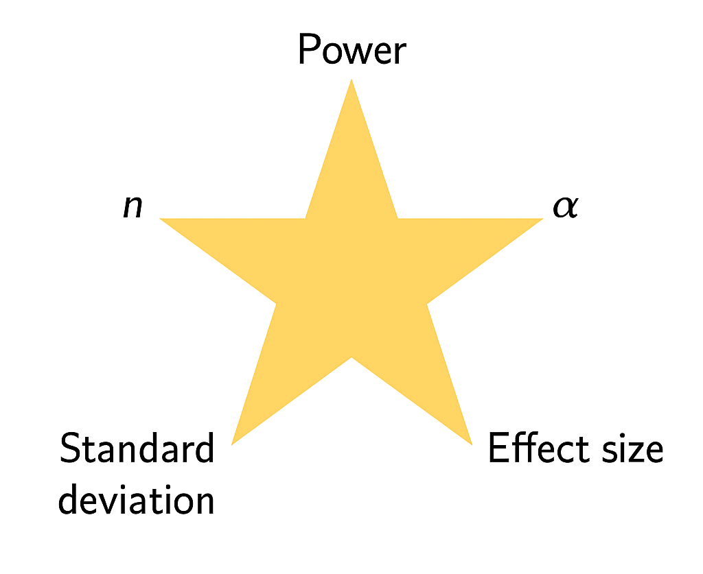
Components of Power Analysis
Motivation: Comparisons of Interest
| Predictor Type | Outcome Type | Common Tests / Topics |
|---|---|---|
| Categorical | Categorical | Fisher’s exact test, \(\chi^2\) test |
| Categorical | Continuous | t-tests, ANOVA, nonparametric alternatives |
| Continuous | Continuous | Correlation*, regression ** |
| Continuous | Categorical | Logistic regression, classification ** |
| Other / Complex | Various (e.g. survival, counts) | Advanced or “exotic” methods ** |
* = covering today
** = covering in upcoming lectures
Remember this plot?
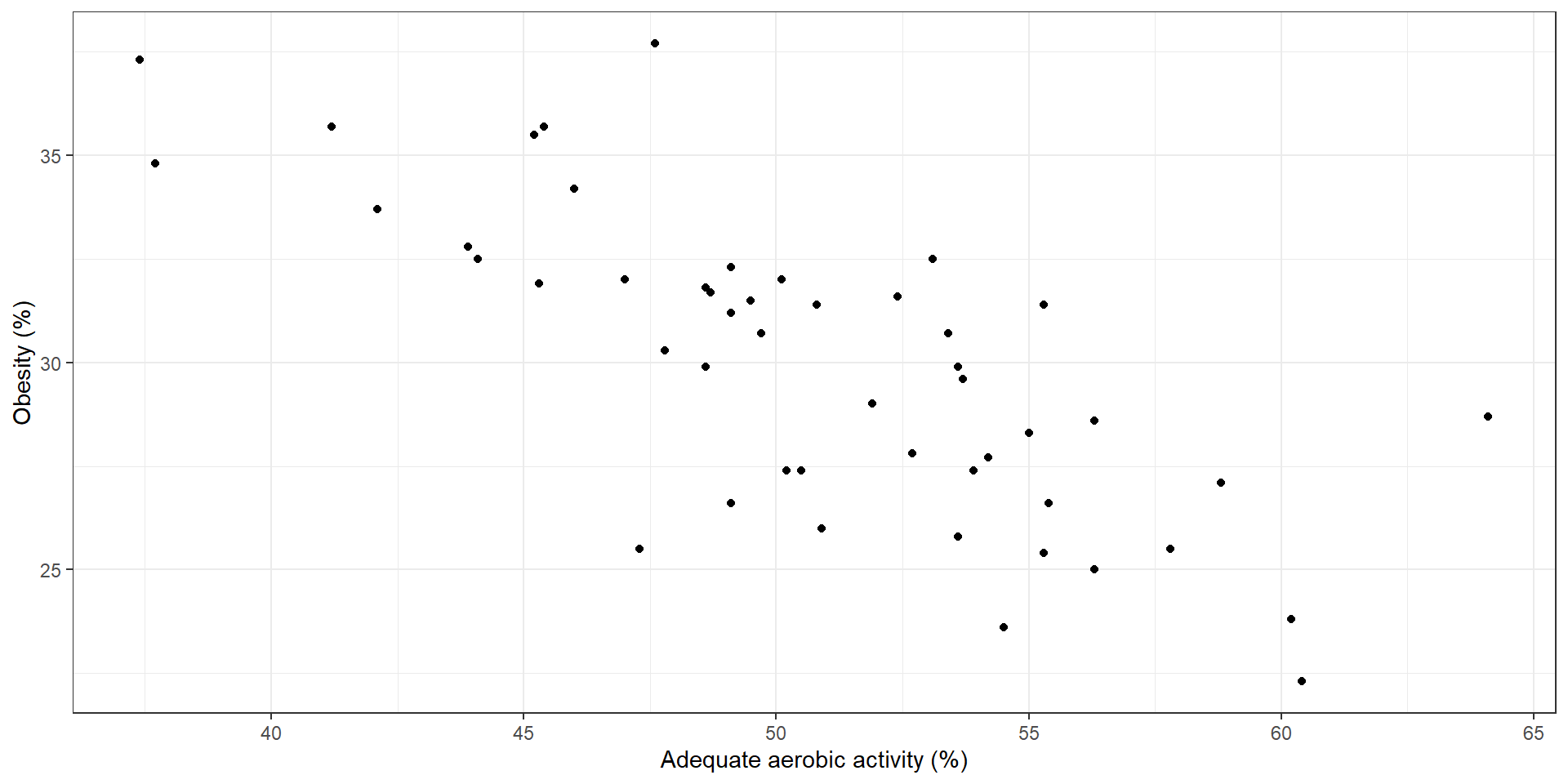
Some questions of interest may include:
Direction of relationship: are variables positively or negatively related?
Form: is any relationship linear or more complex?
Strength of relationship: how accurately can one variable predict the other?
Influential points: are one or a few points driving the relationship we see?
Correlation
The correlation coefficient \(\rho\) quantifies the linear relationship between two random variables.
In statistics, a correlation coefficient implies a very specific type of association.
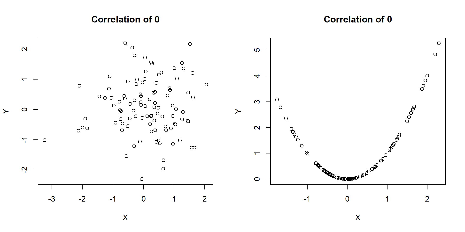
A correlation coefficient of zero does NOT imply no relationship between two variables, as we shall see in some further examples.
Correlation
\(\rho\) ranges from -1 to 1
\(\rho>0\) implies positive correlation
\(\rho < 0\) implies negative correlation
\(\rho = 0\) is consistent with no linear relationship between variables (again, this does not imply that no relationship exists!)
What does it mean to have a correlation of -1 or 1?
Visualizing \(\rho\)
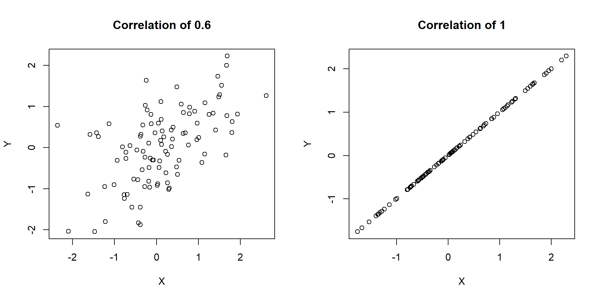
Visualizing \(\rho\)
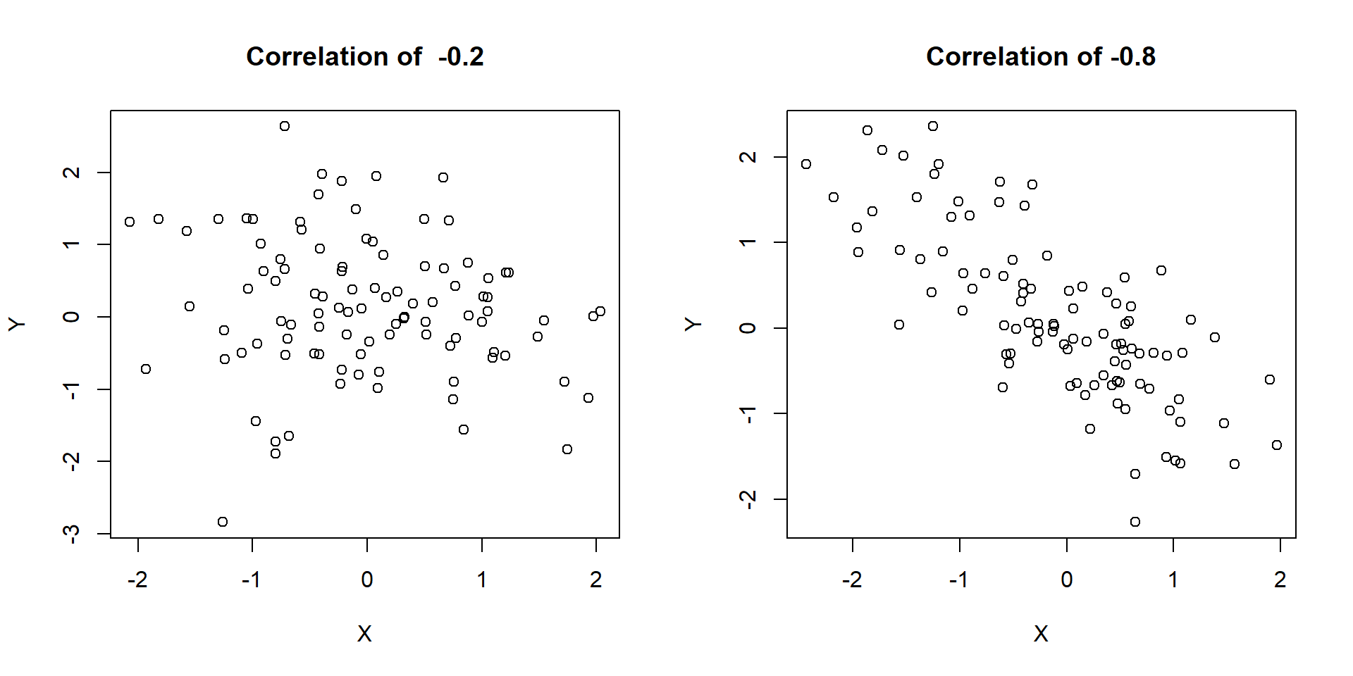
Visualizing \(\rho\)
Pearson’s correlation coefficient
Pearson’s correlation \(r\) gives and estimate of \(\rho\) as follows. Assuming our observed data are the pairs \((x_1, y_1), (x_2, y_2), \ldots, (x_n, y_n)\), we can calculate \(r\) as
\[r = \frac{1}{n} \sum_{i=1}^n \left(\frac{x_i - \bar{X}}{S_x}\right)\left(\frac{y_i - \bar{Y}}{S_y}\right)\]
\[= \frac{\sum_{i=1}^n (x_i - \bar{X})(y_i - \bar{Y})}{\sqrt{\sum_{i=1}^n (x_i - \bar{X})^2\sum_{i=1}^n(y_i - \bar{Y})^2}}\]
No need to memorize this!…we’ll just use the cor() function to calculate it in R.
Anscombe’s quartet
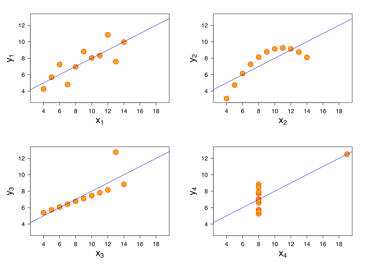
Anscombe’s quartet
In each of the datasets the following statistical summaries hold:
mean of
x: 9variance of
x: 11mean of
y: 7.5variance of
y: 4.125correlation between
xandy: 0.816
Takeaway
Takeaway: Visualizing your data is important! Summary statistics alone cannot capture the full relationship between x and y.
Also, Datasaurus Dozen!
Correlation does not imply causation

Source: Tyler Vigen, Spurious Correlations
Confounding
Many of these spurious correlations are due to confounding - when a third lurking variable is responsible for the observed relationship.
Example: A near perfect negative correlation (r = -0.99) was seen between cholera mortality and elevation above sea level during a 19th century epidemic.
The observed relationship between cholera and elevation was confounded by a lurking variable, proximity to polluted water.
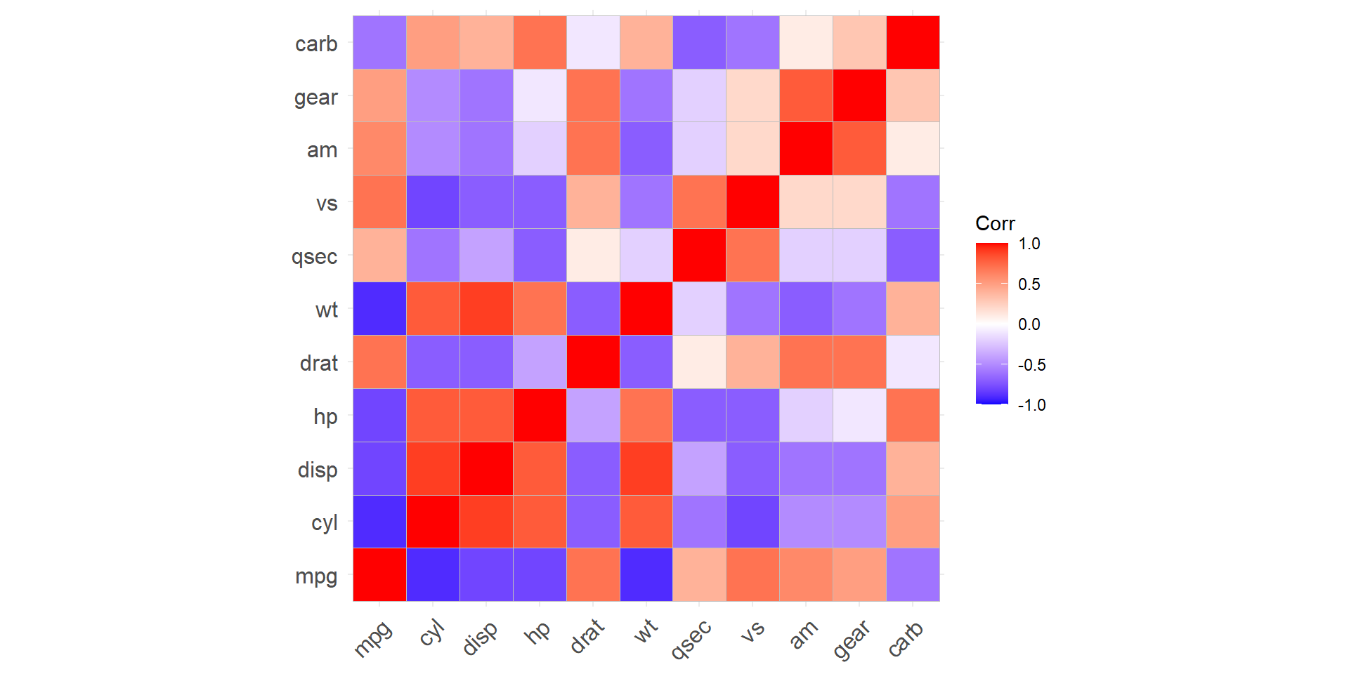
ggcorrplot
ggcorrplotis a fantastic function for making correlation plots in R.This function is in the
ggcorrplotpackage.
- Let’s check out some examples.
Example
mtcarsis a built-in R dataset, taken from the 1974 Motor Trend US magazine. It has fuel consumption and 10 aspects of automobile design/performance for 32 automobiles.mtcarsis built into R, and I can just load the dataset
                   mpg cyl disp  hp drat
Mazda RX4         21.0   6  160 110 3.90
Mazda RX4 Wag     21.0   6  160 110 3.90
Datsun 710        22.8   4  108  93 3.85
Hornet 4 Drive    21.4   6  258 110 3.08
Hornet Sportabout 18.7   8  360 175 3.15
Valiant           18.1   6  225 105 2.76
Example
mtcarsis a built-in R dataset, taken from the 1974 Motor Trend US magazine. It has fuel consumption and 10 aspects of automobile design/performance for 32 automobiles.
      mpg  cyl disp   hp drat   wt
mpg   1.0 -0.9 -0.8 -0.8  0.7 -0.9
cyl  -0.9  1.0  0.9  0.8 -0.7  0.8
disp -0.8  0.9  1.0  0.8 -0.7  0.9
hp   -0.8  0.8  0.8  1.0 -0.4  0.7
drat  0.7 -0.7 -0.7 -0.4  1.0 -0.7
wt   -0.9  0.8  0.9  0.7 -0.7  1.0
Plotting the correlation: code
Plotting the correlation: output
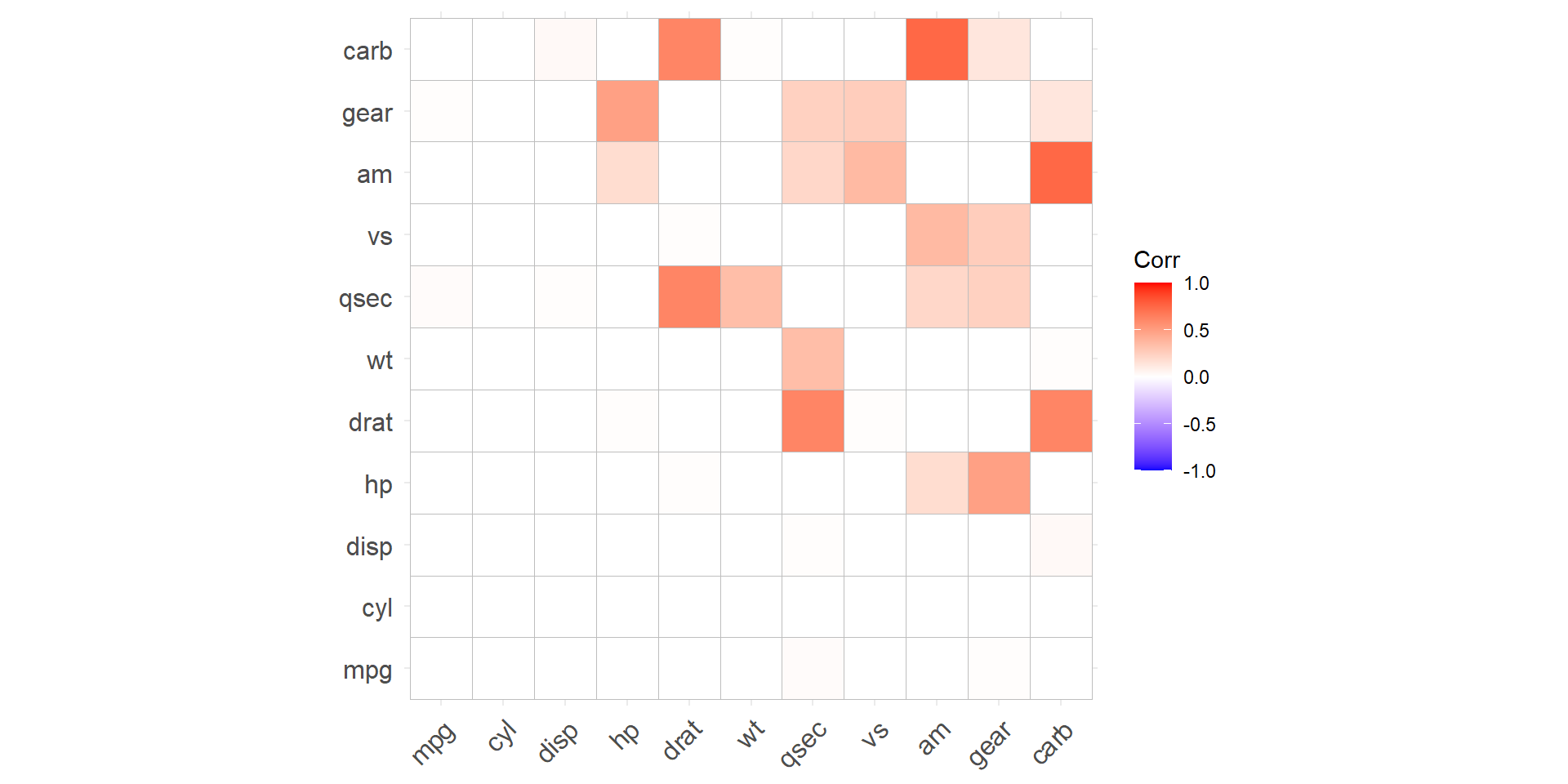
Testing the correlation
- We can also test whether or not each correlation is statistically equal to zero.
\[H_0: \rho = 0 \quad \text{vs.} \quad H_A: \rho \neq 0\]
              mpg          cyl         disp           hp
mpg  0.000000e+00 6.112687e-10 9.380327e-10 1.787835e-07
cyl  6.112687e-10 0.000000e+00 1.802838e-12 3.477861e-09
disp 9.380327e-10 1.802838e-12 0.000000e+00 7.142679e-08
hp   1.787835e-07 3.477861e-09 7.142679e-08 0.000000e+00
drat 1.776240e-05 8.244636e-06 5.282022e-06 9.988772e-03
wt   1.293959e-10 1.217567e-07 1.222320e-11 4.145827e-05
Example: code
R Graph Gallery
R Graph Gallery has lots of examples, with code!
- Along with many other types of plots.
Your turn
AE 05
Head to Canvas and begin working on Application Exercise (AE) 05: Comparing two continuous variables.
AE 05 is due Friday 4/3 at 11:59pm.
Turn in a PDF on Canvas.
Next class
- Review for Exam 02
![]()